
Exploratory Data Analysis
The provided training set contains 1,460 rows and 81 columns — one prediction target (sale price), one ID column, and 79 possible features. Before any modelling, it's important to understand what the data actually looks like.
Feature Distributions
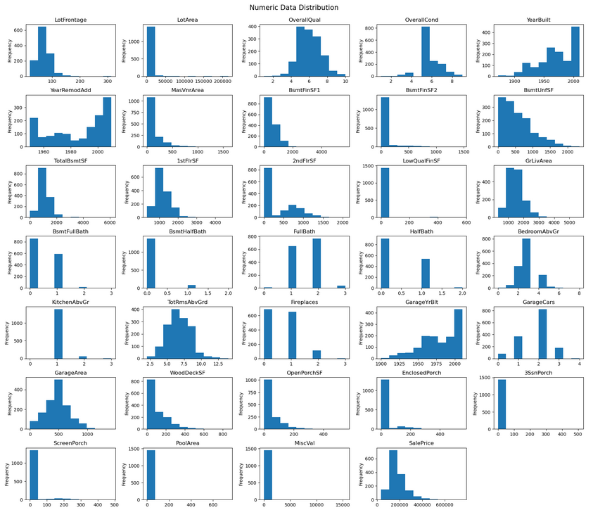
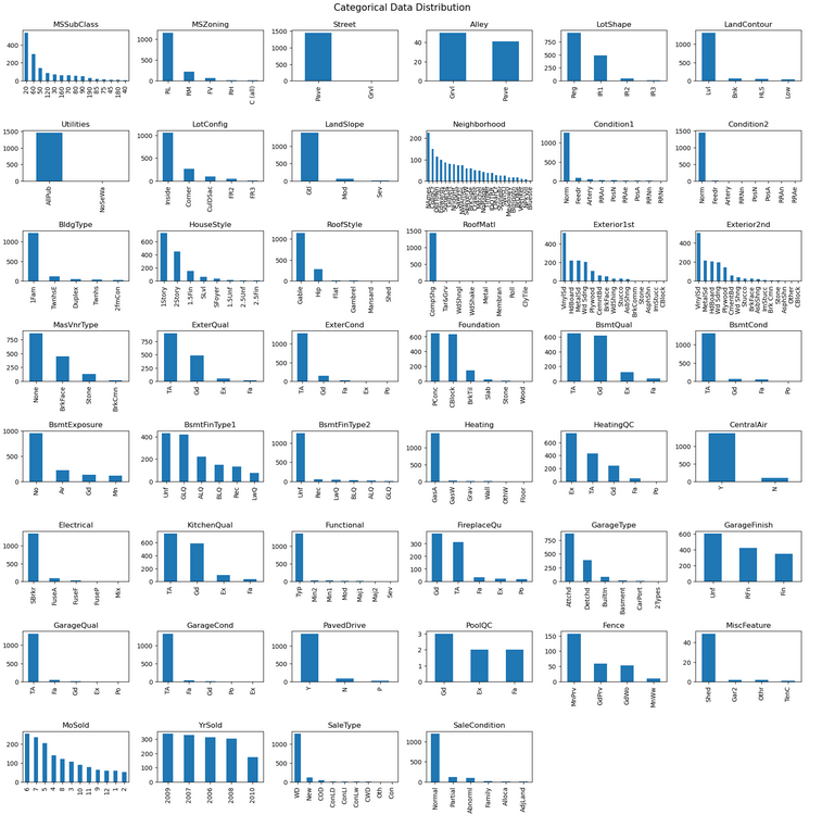
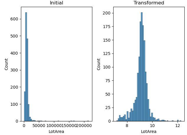
Univariate distributions reveal high skew in several numeric features — BsmtUnfSF is a clear example. Many categorical features also show very uneven distributions: Street is almost entirely "Pave", with "Grvl" appearing only rarely. Features like this offer little predictive value to a model.
Outliers & Correlation
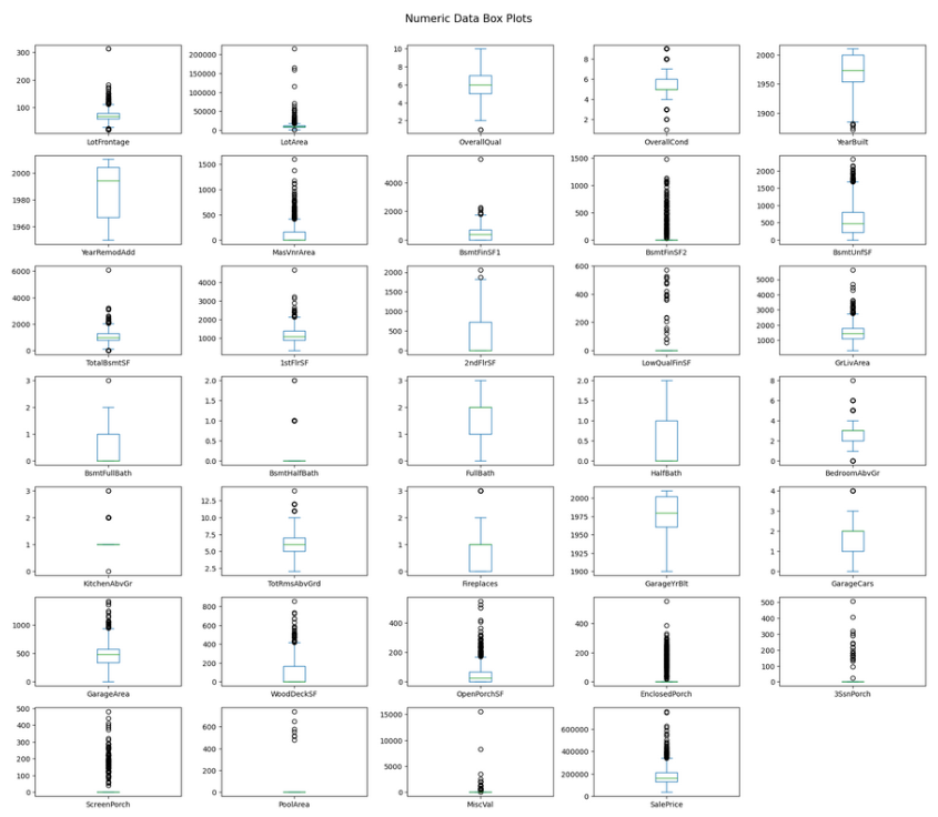
Box plots surface a large number of potential outliers — many caused by the skewed distributions themselves. With only ~1,400 rows, dropping them aggressively would hurt more than help, so most are retained.
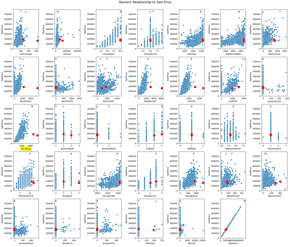
Two specific points in the GrLivArea chart break the otherwise linear relationship between living area and sale price — very large homes sold at unusually low prices, likely anomalies. Removing them strengthens the correlation.
Feature Engineering
With the data understood, the next step is transforming it into a form models can learn from effectively. This involves five stages:
- Handle missing data — Ordinal columns get "NA"; categorical columns take the mode; numeric columns take the median grouped by neighbourhood.
- Add new features — Total bathrooms (upstairs + downstairs) often matters more than either component alone.
- Remove low-signal features — Columns with near-zero correlation or a single value in 99%+ of rows are dropped.
- Transform skewed features — Log transform applied to any feature with skew above 0.5.
- Encode categorical features — Unordered categories use one-hot encoding; ordinal ratings are mapped to integers.
Model Training
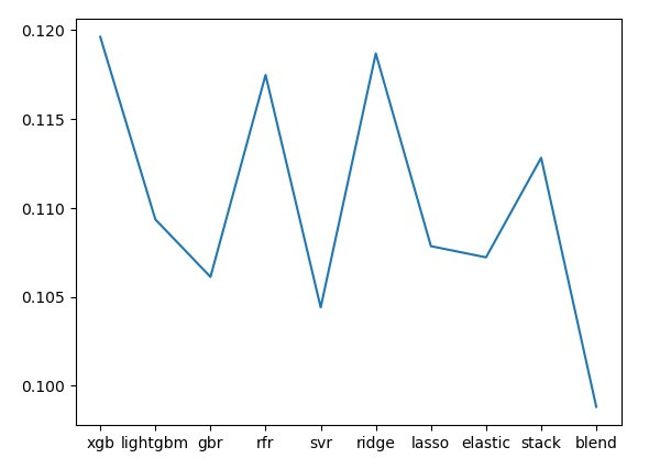
Nine models are trained and evaluated using log RMSE — the Kaggle leaderboard metric. All models are evaluated on a held-out validation set they never saw during training. Individual models cluster between 0.105–0.115. The blended model, combining all nine with optimised weights, reaches 0.099.
Blending approach: 250,000 random weight combinations are tested. The combination with the lowest validation RMSE is kept for the final submission.
Result & what's next
The blended model achieves a top 5% leaderboard finish — well past the original goal of top 10%. Knowing when to stop is itself a useful skill; chasing marginal gains on a competition dataset rarely translates to real-world value.
Areas to revisit if returning to this project:
- Hyperparameter tuning on the individual models
- Proper gradient-based weight optimisation for the blend (currently random search)
- More aggressive feature engineering
- Additional outlier removal based on residual analysis
- Alternative scaling methods (Box-Cox transformation)